x = A b; in Matlab

x = A b;

  1. Is A square?
    no => use QR to solve least squares problem.
  2. Is A triangular or permuted triangular?
    yes => sparse triangular solve
  3. Is A symmetric with positive diagonal elements?
    yes => attempt Cholesky after symmetric minimum degree.
  4. Otherwise
    => use LU on A (:, colamd(A))

Sparse Finite-Element Matrices in MATLAB

March 1st, 2007

Creating Sparse Finite-Element Matrices in MATLAB

I’m pleased to introduce Tim Davis as this week’s guest blogger. Tim is a professor at the University of Florida, and is the author or co-author of many of our sparse matrix functions (lu, chol, much of sparse backslash, ordering methods such as amd and colamd, and other functions such as etree and symbfact). He is also the author of a recent book, Direct Methods for Sparse Linear Systems, published by SIAM, where more details of MATLAB sparse matrices are discussed ( http://www.cise.ufl.edu/~davis ).

Contents

Power iteration

Power iteration

From Wikipedia, the free encyclopedia
In mathematics, the power iteration is an eigenvalue algorithm: given a matrix A, the algorithm will produce a number λ (theeigenvalue) and a nonzero vector v (the eigenvector), such that Av = λv.
The power iteration is a very simple algorithm. It does not compute a matrix decomposition, and hence it can be used when A is a very large sparse matrix. However, it will find only one eigenvalue (the one with the greatest absolute value) and it may converge only slowly.

Krylov subspace

Krylov subspace

From Wikipedia, the free encyclopedia
In linear algebra, the order-r Krylov subspace generated by an n-by-n matrix A and a vector b of dimension n is the linear subspacespanned by the images of b under the first r powers of A (starting from A0 = I), that is,
mathcal{K}_r(A,b) = operatorname{span} , { b, Ab, A^2b, ldots, A^{r-1}b }. ,
It is named after Russian applied mathematician and naval engineer Alexei Krylov, who published a paper on this issue in 1931.[1]
Modern iterative methods for finding one (or a few) eigenvalues of large sparse matrices or solving large systems of linear equations avoid matrix-matrix operations, but rather multiply vectors by the matrix and work with the resulting vectors. Starting with a vector, b, one computes Ab, then one multiplies that vector by A to find A2b and so on. All algorithms that work this way are referred to as Krylov subspace methods; they are among the most successful methods currently available in numerical linear algebra.
Because the vectors tend very quickly to become almost linearly dependent, methods relying on Krylov subspace frequently involve some orthogonalization scheme, such as Lanczos iteration for Hermitian matrices or Arnoldi iteration for more general matrices.
The best known Krylov subspace methods are the ArnoldiLanczosConjugate gradientGMRES (generalized minimum residual),BiCGSTAB (biconjugate gradient stabilized), QMR (quasi minimal residual), TFQMR (transpose-free QMR), and MINRES (minimal residual) methods.

References

  1. ^ Mike Botchev (2002). “A.N.Krylov, a short biography”.

Conjugate gradient method

Conjugate gradient method

From Wikipedia, the free encyclopedia

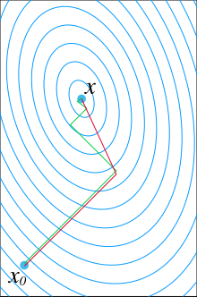
A comparison of the convergence ofgradient descent with optimal step size (in green) and conjugate gradient (in red) for minimizing a quadratic function associated with a given linear system. Conjugate gradient, assuming exact arithmetics, converges in at most n steps where n is the size of the matrix of the system (here n=2).

In mathematics, the conjugate gradient method is an algorithm for the numerical solution of particular systems of linear equations, namely those whose matrix issymmetric and positive-definite. The conjugate gradient method is an iterative method, so it can be applied to sparse systems that are too large to be handled by direct methods such as the Cholesky decomposition. Such systems often arise when numerically solvingpartial differential equations.
The conjugate gradient method can also be used to solve unconstrained optimizationproblems such as energy minimization.
The biconjugate gradient method provides a generalization to non-symmetric matrices. Various nonlinear conjugate gradient methods seek minima of nonlinear equations.